What we need

Well, to learn our CNN we need some basic knowledge in machine learning and programming, we will use the following tools:

1. Python as a main programming language
2. PyTorch as a machine learning framework
3. Google colaboratory as a platform for learning neural network
4. BossBase v.1.01 as a dataset for learning neural network

Retrospective

In the previous part we have a look into theoretical part of the problem. Now let's use this knowledge. If you do not understand what this is about, drink a cup of coffee please refer to the first part.

Data preparation

1) Source grayscale images have 515x512 resolution, but our network will use images with 256x256 resolution. So, lets create a script to resize images.

import cv2

# infrostructure code

for f in listFiles:
    filePath = os.path.join(path, f)

    img = cv2.imread(filePath, -1)
    res = cv2.resize(img, (256, 256))
    cv2.imwrite(f'{outputFolder}/{f}', res)
    idx += 1

After executing image_resizer.py you can make sure that converted images have 256x256 resolution, it's enough to upload an image here.

2) So, we have 10.000 cover grayscale images. We need to embed the date inside each of them. To do that download hugo implementation for your platform and copy all cover images to /images_cover folder. After that execute HUGO_like.exe from /executable folder.

3) If you did all right you should have 10.000 cover and 10.000 stego images. Put them to /cover and /stego respectively. Zip the folder and upload to your Google drive. Data set is ready!

cnn-in-steganalysis/
    ├─cover/
    ├─stego/

4) Retrieve uploaded file id that essential for the next step.

• right click on the file, choose 'get the link' options
• save your unique id

Google colaboratory

To learn our network recognize stego and cover images we need a lot of calculations. Instead of use our own resources (GPU time) we will use Google's resources. It's nice that Google provides powers for young data scientists 👾. Of course, it's possible to use a local machine with a graphic card.

For free use, up to 12 hours are provided every day, but this number can be different and vary depends on the input load. Most probably you won't have enough time to train the network in one pass.

Set up Google colaboratory

First of all, create a new notebook cnn_in_steganalysis.py where we place a code of our future network and make sure that you are using GPU/TPU as a hardware accelerator.

We should mount the driver to have a possibility to save our pretrained network. To mount your Google driver just type and execute the code snippet below. Files from your driver should be available after execution.

from google.colab import drive
drive.mount('/content/gdrive')

Upload and unpack the data set on your virtual machine. From a console execute the code snippet below. Images will be accessible by /content/your_data_set_name path.

!gdown --id your_data_set_id
!unzip your_data_set_name.zip

Define model

The proposed model architecture was described in the first part of this article. Please, refer the first part to get more details. Now we are going to implement it in terms of Pytorch.

Preprocessing

Let's start from preprocessing module that include only one element - HPF filter that uses 30 basic high pass filters from SRM. Our main point here to extract the noise component residuals.

# Image preprocessing
# High-pass filters (HPF)
class HPF(nn.Module):
    def __init__(self):
        super(HPF, self).__init__()
        weight_3x3 = nn.Parameter(torch.Tensor(normalized_hpf_3x3_list).view(25, 1, 3, 3), requires_grad=False)
        weight_5x5 = nn.Parameter(torch.Tensor(normalized_hpf_5x5_list).view(5, 1, 5, 5), requires_grad=False)

        self.preprocess_3x3 = nn.Conv2d(1, 25, kernel_size=(3, 3), bias=False)
        with torch.no_grad():
            self.preprocess_3x3.weight = weight_3x3
            
        self.preprocess_5x5 = nn.Conv2d(1, 30, kernel_size=(5, 5), padding=(1, 1), bias=False)
        with torch.no_grad():
            self.preprocess_5x5.weight = weight_5x5

    def forward(self, x):
        processed3x3 = self.preprocess_3x3(x)
        processed5x5 = self.preprocess_5x5(x)

        # concatenate two tensors
        #   in:  torch.Size([2, 1,256,256])
        #   out: torch.Size([2, 30, 254, 254])
        output = torch.cat((processed3x3, processed5x5), dim=1)
        output = nn.functional.relu(output)

        return output

In forward method we summarize two parts of the residuals to form an output. Then the output will be consumed by the network.

Convolutional module

After preprocessing module we got to the convolutional module. It has 2 separable convolutional and 5 base blocks. Also, this module uses 30 basic high pass filters, all of them available in a repository.

Separable convolutional blocks can be represented as it shown here:

self.separable_convolution_1 = nn.Sequential(
    nn.Conv2d(30, 60, kernel_size=(3, 3), padding=(1, 1), groups=30),
    ABS(),
    nn.BatchNorm2d(60),
    nn.Conv2d(60, 30, kernel_size=(1, 1)),
    nn.BatchNorm2d(30),
    nn.ReLU()
)
# block 2,3
self.base_block_4 = nn.Sequential(
    nn.Conv2d(64, 128, kernel_size=(3, 3), padding=(1, 1)),
    nn.BatchNorm2d(128),
    nn.ReLU(),
    nn.AdaptiveAvgPool2d((1, 1))
)

And base blocks:

self.base_block_1 = nn.Sequential(
    nn.Conv2d(30, 30, kernel_size=(3, 3), padding=(1, 1)),
    nn.BatchNorm2d(30),
    nn.ReLU(),
    nn.AvgPool2d(3, stride=2, padding=1)
)

Everywhere in preprocess module we use Batch Normalization and Rectified Linear Unit activation function because of its effectiveness.

Classification module

Features extracted from the previous module consumed by the classification module. This module consists of three fully connected layers. The first and the second layers has 256 and 1024 neurons. Last layer has only 2 neurons, because there are only two classes - cover and stego image.

self.fc1 = nn.Linear(128, 256)
self.fc2 = nn.Linear(256, 1024)
self.fc3 = nn.Linear(1024, 2)

After the last fully connected layer a softmax activation function is used. It helps distribute network output between [0;1] range, i.e. determine the probability of belonging to one of the classes.

Learning process

After the network has been created and all infrastructure code is done we can start learning. Just click Runtime -> run all in your .py file. After the learning process has been initiated you can see learning progress in the console.

After some epoch (in my experience the number of epoch should be >= 100) stop the script and check your pretrained model by executing acc_and_loss.py script. If you satisfy with the result, you can test the model with real data or continue learning, possibly with new hyper parameters.

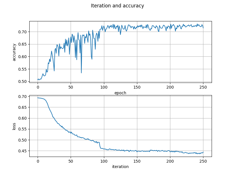
Figure 1. Accurracy and losses

Testing with real data

Ok. We have created a model and spent some time training it... It's time to test our network. To achieve that I propose to create a simple python script that takes input images and process them through the model.

def predict(pretrained_model_path, image_path):
    # do some checks here
    ...
    
    final_json = {}
    
    # load network
    net = CnnSteganalysis()
    loaded_state = torch.load(pretrained_model_path, map_location='cpu')['model_state']
    with torch.no_grad():
        # load state and enable evaluate
        net.load_state_dict(loaded_state)
        net.eval()
        if os.path.isdir(args.image):
            images = os.listdir(args.image)
            for idx, val in enumerate(images):
                output = proceed(image_path + '/' + val, net)
                interpret_prediction(output, val, final_json, idx)
        else:
            output = proceed(image_path, net)
            interpret_prediction(output, image_path, final_json)

    print(json.dumps(final_json))


def proceed(path_to_image, net):
    # read image and process through the network
    ...
    output = net(img_array)
    return output


def interpret_prediction(output, image_name, history, idx=0):
    prediction = output.max(1, keepdim=True)
    prediction_tensor = prediction[1]

    cover_percentage, stego_percentage = output[0].numpy()
    if prediction_tensor[0].numpy()[0] == 0:
        history[idx] = {
            'imageName': os.path.basename(image_name),
            'probability': f'{cover_percentage:.4f}/{stego_percentage:.4f}',
            'result': 'COVER'
        }
    else:
        history[idx] = {
            'imageName': os.path.basename(image_name),
            'probability': f'{cover_percentage:.4f}/{stego_percentage:.4f}',
            'result': 'STEGO'
        }

Instead of conclusion

All hyper parameters can be found in final .py file. At this topic we implemented experimental network that can classify image as cover or stego image. Of course, it's just an example some of the parts proposed network can be improved.

All infrastructure code is deliberately missed and available in a repository.

Finally, you can find final .py file and other code here. 🎉🎉🎉